DSA Bloom

What is a Data Structure?

A Data Structure is a way to organize and store data in a computer so it can be used easily.

For example, a program may store:
numbers,names, messages, images
If data is not organized, the computer cannot work with it efficiently.

So we use data structures to store and manage data properly.

Why Do We Need Data Structures?

Data structures help us to:

1. Store data efficiently
2. Find data quickly
3. Update data easily
4. Process large amounts of data
5. Without data structures, programs would become slow and difficult to manage.
6. Big systems like social media, banking apps, and search engines all use data structures.

Types of Data Structures?

There are many kinds of data structures. The most common ones are:

Basic Data Structures
Array
Linked List
Stack
Queue

Advanced Data Structures
Tree
Graph
Hash Table
Heap

We will learn each one step by step with examples and code.

What is an Array?

An Array is a data structure used to store multiple values in one variable.
Instead of creating many variables, we store everything inside one array.

Example:
let numbers = [10, 20, 30, 40];
Here the array stores 4 values.

Array Index

Each value in an array has a position number called an index.

Important rule:
Array index always starts from 0

Example:
let numbers = [10, 20, 30, 40];
Index Value
0 - 10
1 - 20
2 - 30
3 - 40

Accessing values:
numbers[0] → 10
numbers[2] → 30

Basic Array Operations

Common things we do with arrays:

1 Access value
numbers[1]

2 Add value
numbers.push(50)

3 Remove value
numbers.pop()

4 Change value
numbers[0] = 100

Arrays are very fast for accessing data using index.

What is Time Complexity?

Time Complexity means:
How much time a program takes to run

We don’t measure time in seconds.
We measure how the time grows when input increases.

Example idea:
Small data → fast
Big data → slower

Time complexity helps us understand how efficient our code is.

Big O Notation:

We use something called Big O Notation to describe time complexity.

It looks like this:

O(1) → very fast (constant time)
O(n) → grows with input
O(n²) → slower (nested loops)

Example:
for(let i = 0; i < n; i++){
console.log(i);
}

This is O(n) because it runs n times.

Common Time Complexities:

Here are the most important ones:

⚡ O(1) – Constant
Always same speed
Example:
numbers[0]

🚶 O(n) – Linear
Depends on input size
Example:
for(let i = 0; i < n; i++){}

🐢 O(n²) – Quadratic
Very slow for big data
Example:
for(let i = 0; i < n; i++){
for(let j = 0; j < n; j++){}
}

💡 Simple idea:
O(1) → best
O(n) → okay
O(n²) → avoid if possible

What is a Linked List?

A Linked List is a data structure where:
👉 Each item (node) is connected to the next item

It is like a chain:
[10] → [20] → [30] → [40]
Each part is called a node.

Structure of a Node:

Structure of a Node

Each node has 2 parts:

1 Data → the value (like 10, 20)
2 Next → a link to the next node

Example:
let node = {
data: 10,
next: null
}

Chain example:
10 → 20 → 30 → null
👉 null means end of list

Linked List vs Array:

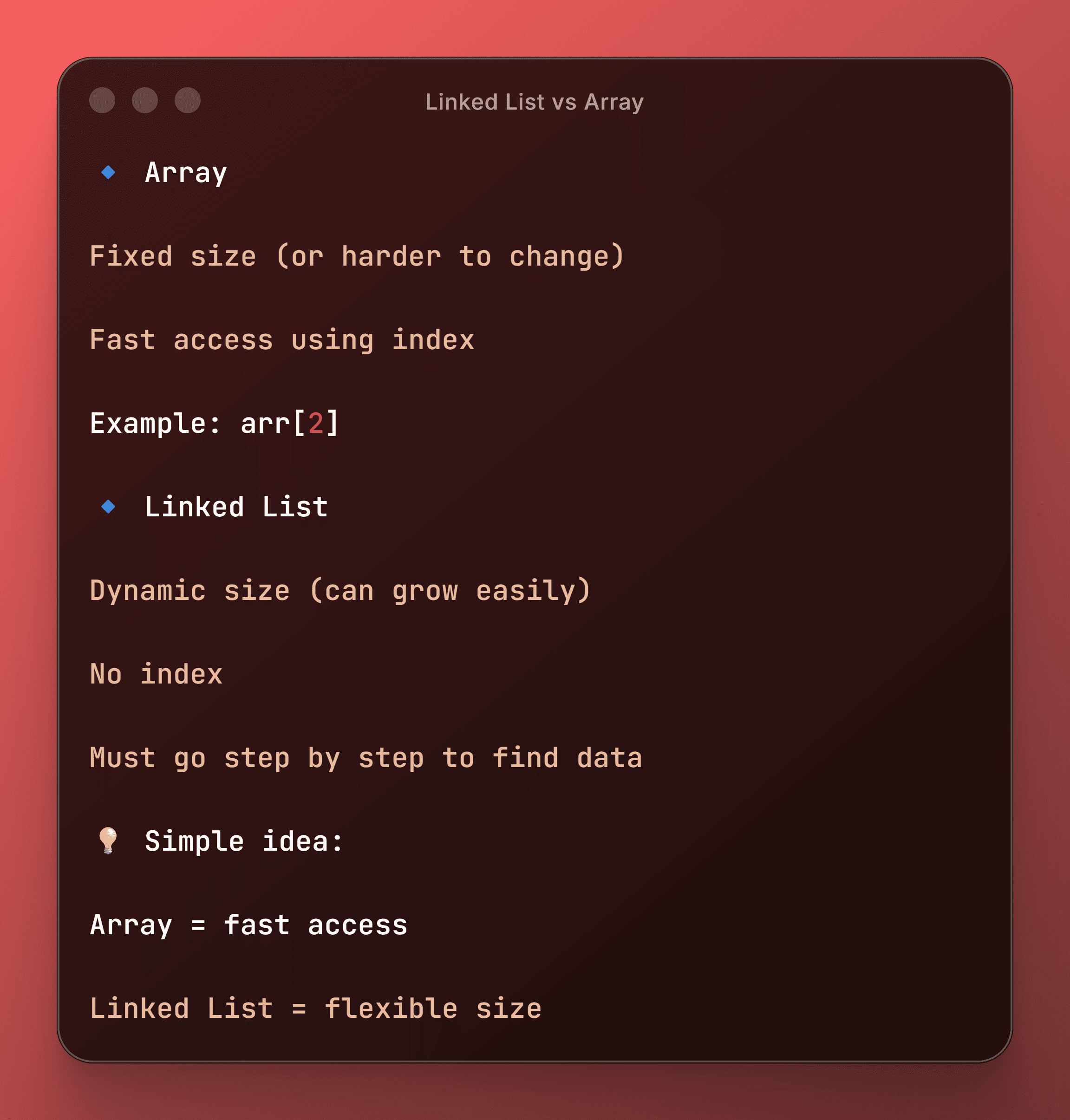
Array
Fixed size (or harder to change)
Fast access using index
Example: arr[2]

Linked List
Dynamic size (can grow easily)
No index
Must go step by step to find data

💡 Simple idea:
Array = fast access
Linked List = flexible size

Traversing a Linked List:

Traverse means:

👉 Go through all nodes one by one
Since there is no index, we must start from the beginning.

Example:
let current = head;
while(current !== null){
console.log(current.data);
current = current.next;
}
💡 This prints all values in the list.

Inserting Data into a Linked List:

👉 Insert at beginning
let newNode = {
data: 5,
next: head
};
head = newNode;
Now list becomes:
5 → 10 → 20 → 30

👉 Insert at end
let newNode = {
data: 50,
next: null
};
let current = head;
while(current.next !== null){
current = current.next;
}
current.next = newNode;

Deleting Data from a Linked List:

👉 Delete first node
head = head.next;

👉 Delete specific value
let current = head;
while(current.next !== null){
if(current.next.data === 20){
current.next = current.next.next;
break;
}
current = current.next;
}

💡 Simple idea:
Traverse → read data
Insert → add node
Delete → remove node

What is a Stack?

A Stack is a data structure that follows:
👉 LIFO (Last In, First Out)

Meaning:
The last item you add is the first one you remove

Example:
[10, 20, 30]
👉 30 will be removed first

Stack Operations:

1 Push (Add item)
stack.push(40)
Now:
[10, 20, 30, 40]

2 Pop (Remove item)
stack.pop()
Removes 40

3 Peek (See top item)
stack[stack.length - 1]
Shows last value without removing it
💡 Stack always works from the top

What is a Queue?

A Queue is a data structure that follows:
👉 FIFO (First In, First Out)

Meaning:
First item added is the first one removed

Example:
[10, 20, 30]
👉 10 will be removed first

Queue Operations:

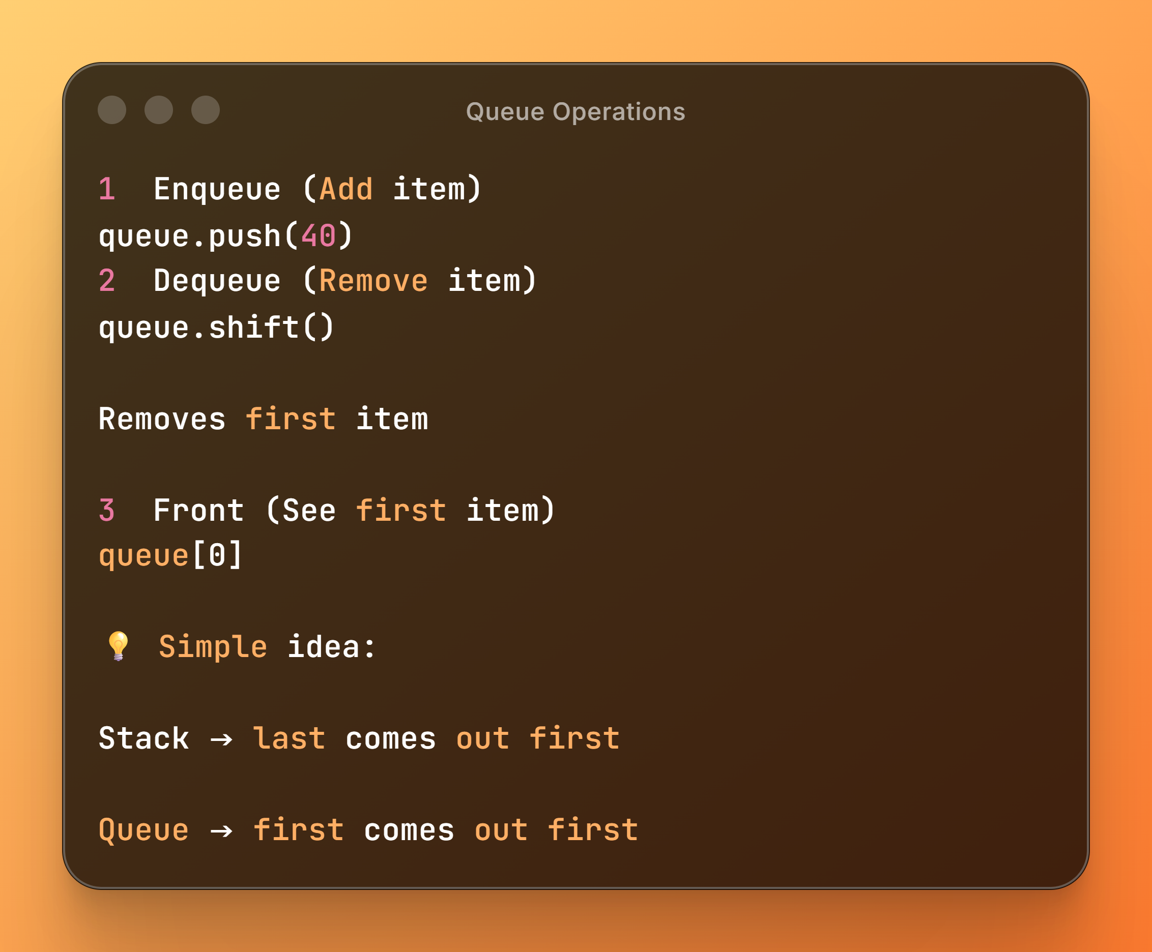
1 Enqueue (Add item)
queue.push(40)

2 Dequeue (Remove item)
queue.shift()
Removes first item

3 Front (See first item)
queue[0]

💡 Simple idea:
Stack → last comes out first
Queue → first comes out first

What is a Tree?

A Tree is a data structure that looks like a hierarchy.
It starts from one top node and branches down.
Example:
10
/   \
20 30
/  \
40 50

Important Terms:
Root → top node (10)
Parent → node with children (20)
Child → node below (40, 50)
Leaf → node with no children (40, 50, 30)

💡 Trees are used in:
File systems
Databases
Searching

Binary Tree:

A Binary Tree is a tree where:
👉 Each node can have maximum 2 children
Left child
Right child
Example:
10
/   \
20 30

💡 Rule:
Each node → at most 2 children

Queue Operations:

A BST is a special binary tree with rules:
👉 Left side → smaller values
👉 Right side → bigger values
Example:
10
/   \
5   20
/  \   \
2   7   30
Why BST is powerful?

Because it makes searching very fast
👉 Like binary search

Tree Traversal:

Traversal means:
👉 Visiting all nodes
Types:
1 Inorder (Left → Root → Right)
Left → Root → Right

2 Preorder (Root → Left → Right)
Root → Left → Right

3 Postorder (Left → Right → Root)
Left → Right → Root

💡 Traversal is used to:
Read data
Process trees

What is a Graph?

A Graph is a data structure used to show connections between things.
It has:
Nodes (Vertices) → points
Edges → connections between nodes
Example:
A — B
|        |
C — D

💡 Real life examples:
Social networks
Maps (cities & roads)
Internet connections

Types of Graphs:

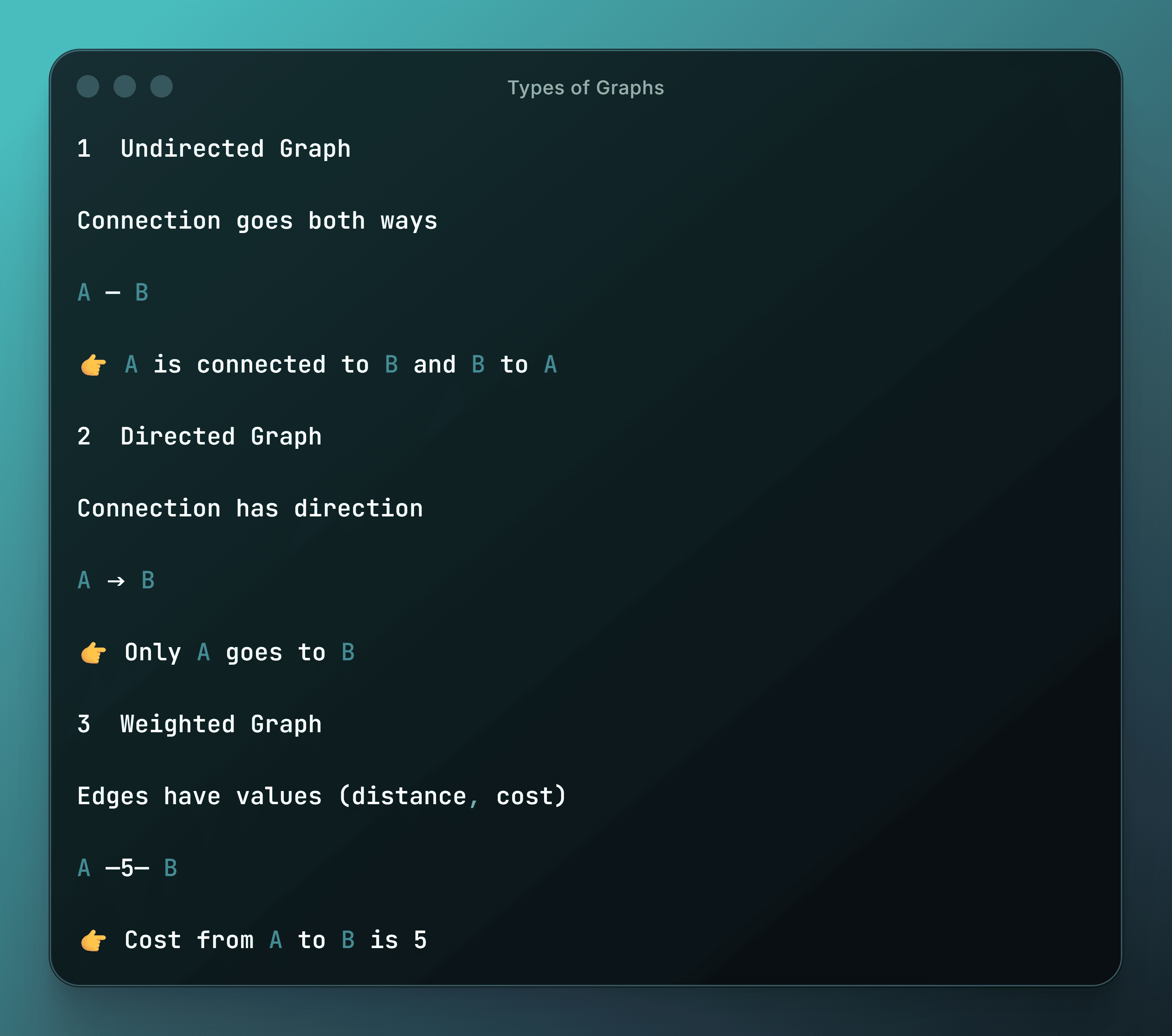
1 Undirected Graph
Connection goes both ways
A — B
👉 A is connected to B and B to A

2 Directed Graph
Connection has direction
A → B
👉 Only A goes to B

3 Weighted Graph
Edges have values (distance, cost)
A —5— B
👉 Cost from A to B is 5

Graph Traversal:

Traversal means:
👉 Visiting all nodes

🔵 BFS (Breadth First Search)
Goes level by level
Uses Queue

Example flow:
A → B → C → D

🔴 DFS (Depth First Search)
Goes deep first
Uses Stack

Example flow:
A → B → D → C

💡 Simple idea:
BFS → wide (level)
DFS → deep

Hash Table:

A Hash Table stores data in key-value pairs.
Example:
{
name: "Zohil",
age: 20
}

Why use Hash Table?
👉 Very fast access
data["name"] // very fast

💡 Used in:
Databases
Caching
APIs

Heap:

A Heap is a special tree used for priority.

Types:

🔹 Min Heap
Smallest value on top

🔹 Max Heap
Largest value on top
Example (Min Heap):
 5
/   \
10  20

💡 Used in:
Priority queues
Scheduling
Algorithms

Sorting Algorithms:

Sorting means:
👉 Arranging data in order (small → big or big → small)

Example:
[5, 2, 9, 1] → [1, 2, 5, 9]

Common Sorting Types:

1 Bubble Sort
Compare and swap values
Simple but slow
👉 Time: O(n²)

2 Selection Sort
Find smallest and place it first
👉 Time: O(n²)

3 Quick Sort (Important)
Divide and sort
👉 Time: O(n log n) (fast)

💡 Simple idea:
Small data → any sort works
Big data → use Quick Sort

Searching Algorithms:

Searching means:
👉 Finding a value

1 Linear Search
Check one by one
for(let i = 0; i < arr.length; i++){
if(arr[i] === x) return i;
}
👉 Time: O(n)

2 Binary Search (Very Important)
👉 Works only on sorted array
Steps:
Check middle
Go left or right
👉 Time: O(log n) (very fast)

Recursion:

Recursion means:
👉 A function calling itself

Example:
function count(n){
if(n === 0) return;
console.log(n);
count(n - 1);
}

💡 Important:
Every recursion must have:
Base case (stop condition)
Recursive call

Practice Problems:

To become strong 💪 you must practice:

Examples:
Reverse array
Find max/min
Palindrome check
Stack/Queue problems
Tree traversal
👉 Practice = real learning

Mini-Project + Interview Prep:

🛠 Mini Project Ideas:
Task Manager (use arrays + stack)
Contact list (use hash table)
Simple search system

Interview Tips:

Understand concepts (not memorize)
Practice coding daily

Focus on:
Arrays
Strings
Trees
Graphs

Congratulations!

What is an Algorithm?

An Algorithm is:
👉 A step-by-step process to solve a problem

Example:
Problem: Make tea ☕
Algorithm:

1. Boil water
2. Add tea
3. Add sugar
4. Pour into cup

💡 In programming:
Algorithm = steps your code follows

Why Algorithms Matter?

Algorithms help you:

Solve problems correctly
Make programs faster ⚡
Handle big data easily
Write better code
👉 Same problem, different algorithm → different speed

Algorithm vs. Data Structure

👉 Data Structure = how data is stored
👉 Algorithm = how data is used

Example:
Array (data structure)
Searching in array (algorithm)

💡 Simple idea:
Data Structure = container
Algorithm = action

Types of Algorithms:

There are different types of algorithms based on how they solve problems:

🔹 1. Brute Force
👉 Try every possible solution
Example:
Check each number one by one
💡 Simple but slow

🔹 2. Divide and Conquer
👉 Break problem into smaller parts
Example:
Binary Search
Quick Sort
💡 Very fast and powerful

🔹 3. Greedy Algorithm
👉 Pick the best choice at each step
Example:
Choosing biggest profit first
💡 Fast but not always correct

🔹 4. Dynamic Programming (DP)
👉 Solve once, store result, reuse it
💡 Saves time, avoids repeating work

Algorithm Efficiency:

Efficiency means:
👉 How fast and how much memory an algorithm uses

We measure:
Time Complexity (speed)
Space Complexity (memory)

💡 Goal:
👉 Use less time + less memory

Input and Output:

Every algorithm has:

👉 Input
Data given to algorithm
Example:
[1, 2, 3]

👉 Output
Result after processing
Example:
[3, 2, 1]

💡 Simple idea: Input → Process → Output

Linear Search Algorithm:

Linear Search means:

👉 Check each element one by one until you find the target
Example:

[10, 20, 30, 40]
Find: 30
Steps:
Check 10 ❌
Check 20 ❌
Check 30 ✅ (found)

Code:

function linearSearch(arr, target){
for(let i = 0; i < arr.length; i++){
if(arr[i] === target){
return i;
}
}
return -1;
}

👉 Time: O(n)

Binary Search Algorithm:

Works only on sorted arrays

Example:
[10, 20, 30, 40, 50]
Find: 30
Steps:
Check middle → 30 ✅ found

Code:
function binarySearch(arr, target){
let left = 0;
let right = arr.length - 1;
while(left <= right){
let mid = Math.floor((left + right) / 2);
if(arr[mid] === target){
return mid;
} else if(arr[mid] < target){
left = mid + 1;
}
else{
right = mid - 1;
}
}
return -1;
}

👉 Time: O(log n) (very fast)

Bubble Sort Algorithm:

👉 Compare and swap adjacent values

Example:
[5, 3, 2]
Steps:
5 ↔ 3 → [3,5,2]
5 ↔ 2 → [3,2,5]
3 ↔ 2 → [2,3,5]

Code:

function bubbleSort(arr){
for(let i = 0; i < arr.length; i++){
for(let j = 0; j < arr.length - i - 1; j++){
if(arr[j] > arr[j + 1]){
let temp = arr[j];
arr[j] = arr[j + 1];
arr[j + 1] = temp;
}
}
}
return arr;
}

👉 Time: O(n²) (slow)

💡 Simple idea:
Linear → check all
Binary → smart search
Bubble → simple sorting

Selection Sort:

👉 Idea:
Find the smallest value and put it at the beginning.

Example:
[5, 3, 2, 4]
Steps:
Smallest = 2 → swap with 5 → [2,3,5,4]
Next smallest = 3 → already correct
Next smallest = 4 → swap with 5 → [2,3,4,5]
Code:
function selectionSort(arr){
for(let i = 0; i < arr.length; i++){
let minIndex = i;
for(let j = i + 1; j < arr.length; j++){
if(arr[j] < arr[minIndex]){
minIndex = j;
}
}
let temp = arr[i];
arr[i] = arr[minIndex];
arr[minIndex] = temp;
}
return arr;
}
👉 Time: O(n²)

Insertion Sort:

👉 Idea:

Pick one element and insert it in the correct position
Example:
[5, 3, 4]
Steps:
Take 3 → place before 5 → [3,5,4]
Take 4 → place between → [3,4,5]
Code:
function insertionSort(arr){
for(let i = 1; i < arr.length; i++){
let key = arr[i];
let j = i - 1;
while(j >= 0 && arr[j] > key){
arr[j + 1] = arr[j];
j--;
}
arr[j + 1] = key;
}
return arr;
}
👉 Time: O(n²) (but faster than bubble in practice)

Merge Sort (Important):

👉 Uses Divide & Conquer

Steps:
Divide array into halves
Sort each half
Merge them
Example:

[5, 3, 2, 4]
→ [5,3] [2,4]
→ [3,5] [2,4]
→ [2,3,4,5]

Code:

function mergeSort(arr){
if(arr.length <= 1) return arr;
let mid = Math.floor(arr.length / 2);
let left = mergeSort(arr.slice(0, mid));
let right = mergeSort(arr.slice(mid));
return merge(left, right);
}
function merge(left, right){
let result = [];
let i = 0, j = 0;
while(i < left.length && j < right.length){
if(left[i] < right[j]){
result.push(left[i]);
i++;
} else {
result.push(right[j]);
j++;
}
}
return result.concat(left.slice(i)).
concat(right.slice(j));
}

👉 Time: O(n log n) (fast)
💡 Simple idea:

Selection → find smallest
Insertion → place correctly
Merge → divide and combine

Quick Sort (Important):

👉 Uses Divide & Conquer like Merge Sort

Steps:
Pick a pivot
Place smaller values on left, bigger on right
Recursively sort left and right
Example:

[5, 3, 8, 4, 2]
Pivot = 5
Left: [3,4,2], Right: [8]
Sort Left → [2,3,4]
Combine → [2,3,4,5,8]

Code:

function quickSort(arr){
if(arr.length <= 1) return arr;
let pivot = arr[arr.length - 1];
let left = [], right = [];
for(let i = 0; i < arr.length - 1; i++){
if(arr[i] < pivot) left.push(arr[i]);
else right.push(arr[i]);
}
return [...quickSort(left), pivot, ...quickSort(right)];
}

👉 Time: O(n log n) average, O(n²) worst
💡 Very fast in practice

Recursion Deep Dive:

Recursion = function calling itself

Important rules:
Base case → stop condition
Recursive call → keep going

Example: Factorial

function factorial(n){
if(n === 0) return 1;
return n * factorial(n - 1);
}
Factorial of 5 → 5 * 4 * 3 * 2 * 1 = 120

Common Recursion Patterns:

Counting / Summing
Traversing arrays
Tree traversal
Divide & Conquer

Fibonacci Sequence (Recursion Example):

Fibonacci:

0, 1, 1, 2, 3, 5, 8, ...

Recursive Code:
function fib(n){
if(n <= 1) return n;
return fib(n - 1) + fib(n - 2);
}

💡 Simple idea:
Recursion = break big problem into smaller ones

Greedy Algorithm:

Greedy Algorithm = always pick the best choice at the current step.

Example: Coin Change Problem
Coins: 25, 10, 5, 1
Amount: 41

Steps:
Take 25 → Remaining 16
Take 10 → Remaining 6
Take 5 → Remaining 1
Take 1 → Done

💡 Simple and fast, but not always optimal for all problems.

Fractional Knapsack (Greedy Example):

Problem: Pick items to maximize value

Each item has weight and value
Can take fraction of item

Algorithm:
Sort items by value/weight ratio
Pick items starting from highest ratio until full

Code (Simplified):

function fractionalKnapsack(items, W){
items.sort((a,b) => b.value/a.weight - a.value/b.weight);
let total = 0;
for(let item of items){
if(W >= item.weight){
W -= item.weight;
total += item.value;
} else {
total += item.value * (W/item.weight);
break;
}
}
return total;
}

Dynamic Programming (DP) Intro:

Dynamic Programming = solve once, store result, reuse

Used when a problem has:
Overlapping subproblems
Optimal substructure

Example: Fibonacci Sequence
Recursive version = slow
DP version = fast (memoization)

DP Example (Fibonacci with Memoization)
let memo = {};
function fib(n){
if(n in memo) return memo[n];
if(n <= 1) return n;
memo[n] = fib(n-1) + fib(n-2);
return memo[n];
}

💡 Now fib(50) runs instantly instead of very slow recursion.

What is Backtracking?

Backtracking = try all possibilities but undo if wrong

Idea:

Go forward → if it fails → go back → try another path

Example: Maze problem
Go through paths
Dead end → backtrack

N-Queens Problem (Backtracking Example):

Problem: Place N queens on N×N chessboard so no two queens attack each other.

Steps:

Place queen in first row
Move to next row
If safe → continue
If not safe → backtrack

💡 Used in puzzles, combinatorics, and constraint problems

Code (Simplified Pseudo-JS):
You can Check Example in it's picture!!!

Recursion Practice (Important):

Practice problems:

Reverse a string
Sum of array elements
Factorial
Fibonacci
Tree traversal

💡 Key idea:
Solve big problem → break into small problem → combine result

BFS (Breadth First Search):

👉 BFS = visit nodes level by level

Uses Queue
Starts from a node and explores neighbors first

Example:

A → B → C → D

Code:

function bfs(graph, start){
let queue = [start];
let visited = new Set();

while(queue.length > 0){
let node = queue.shift();

if(!visited.has(node)){
console.log(node);
visited.add(node);

for(let neighbor of graph[node]){
queue.push(neighbor);
}
}
}
}

💡 Used in:

Shortest path (unweighted)
Social networks

DFS (Depth First Search):

👉 DFS = go deep first, then back

Uses Stack (or recursion)

Example:

A → B → D → C

Code:

function dfs(graph, node, visited = new Set()){
if(visited.has(node)) return;

console.log(node);
visited.add(node);

for(let neighbor of graph[node]){
dfs(graph, neighbor, visited);
}
}

💡 Used in:
Path finding
Cycle detection

Dijkstra’s Algorithm:

👉 Finds shortest path in weighted graph

Example:

Cities with distances
Steps:
Start from source
Pick smallest distance node
Update neighbors
Repeat

Simple Idea:
Always choose minimum distance

💡 Used in:

Google Maps
Network routing

Difference (BFS vs DFS):

💡 Simple idea:

BFS → wide
DFS → deep

String Algorithms Basics:

A string is just text:

"hello"
Common problems:
Reverse a string
Check palindrome
Count characters
Find substring

Example: Reverse String

function reverse(str){
return str.split('').reverse().join('');
}
Example: Palindrome Check
function isPalindrome(str){
return str === str.split('').reverse().join('');
}

💡 Used in:

Search engines
Text processing
Validation

Sliding Window Technique:

👉 Used for arrays & strings

Idea:

Use a “window” and move it step by step
Avoid re-calculating again and again
Example: Max Sum of Subarray
function maxSum(arr, k){
let sum = 0;

for(let i = 0; i < k; i++){
sum += arr[i];
}

let max = sum;

for(let i = k; i < arr.length; i++){
sum += arr[i] - arr[i - k];
max = Math.max(max, sum);
}

return max;
}

💡 Much faster than checking all subarrays

Two Pointer Technique:

👉 Use two indexes to solve problems

Example:
Find pair with sum = target

function twoSum(arr, target){
let left = 0;
let right = arr.length - 1;

while(left < right){
let sum = arr[left] + arr[right];

if(sum === target) return [left, right];
else if(sum < target) left++;
else right--;
}
}

💡 Works best on sorted arrays

Prefix Sum:

👉 Store cumulative sums to answer queries fast

Example:

let arr = [1,2,3,4];

let prefix = [];
prefix[0] = arr[0];

for(let i = 1; i < arr.length; i++){
prefix[i] = prefix[i-1] + arr[i];
}

💡 Now you can get sum of any range quickly

Bit Manipulation (Basics):

👉 Work with binary (0 and 1)

Example:

5 = 101
3 = 011
AND (&)
5 & 3 = 1

💡 Used in:

Optimization
Competitive programming

Practice Problems (Must Do):

Now the most important step:

👉 Practice = real skill
Start with:

Easy:

Reverse array
Find max/min
Palindrome check
Linear search

Medium:

Two Sum
Sliding window problems
Binary search problems

Hard:

Tree problems
Graph traversal
Dynamic Programming

💡 Rule:

👉 Don’t just read — solve by yourself

Real Problem Solving Strategy:

When you see a problem:

Step 1: Understand problem

👉 What is input? What is output?

Step 2: Think simple solution
👉 Even if slow (brute force)

Step 3: Optimize

👉 Use:

Binary Search
Sliding Window
Hash Table
DP

💡 Always go:

Simple → Better → Best

Interview Preparation:

What companies expect:

Clear thinking
Clean code
Problem solving
Good understanding of basics

Focus topics:

Arrays & Strings
Linked List
Trees
Graphs
Recursion & DP

Tips:

Practice daily (even 1–2 problems)
Explain your thinking
Don’t panic in interview

🎉 CONGRATULATIONS